Safety against uncertain obstacles using probabilistic control barrier function

Chinmay Maheshwari, Jichan Chung, Prasanth Kotaru. EE227BT - Convex Optimization, Fall 2019. Presentation pdf

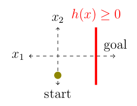
A given dynamical system is said to be safe, if the system states belong to a safe-set, i.e., \(x\in \mathcal{C}, \forall t\geq 0\) [1]. The safety set C is defined as a super-level set of a differential function \(h(x) : \mathbb{R}^n\rightarrow \mathbb{R},\quad \mathcal{C}=\{x: h(x)\geq 0\}\). Typically, \(h(x)\) is a function of system state \(x\) and the environment, for instance, \(h(x) = dist(x, x_{obstacle} )−\varepsilon\).

The objective is to ensure that the state \(x\) belongs to the safety-set with high-probablity. This is achieved using the following optimization formulation,

\[ \begin{align} \min_{(u,\delta)\in\mathcal{U}\times\mathbb{R}} & \quad u^\top u + \delta^2 \label{eq:prcbf} \\ \text{subject to} & \quad L_f V(x) + L_g V(x) u + \gamma V(x) - \delta \leq 0, \\ & \quad Pr(L_fh(x) + L_gh(x)u + \lambda h(x) \geq 0)\geq \eta \quad \text{(PrCBF)} \end{align} \]

For a linear barrier function, \(h = a^Tx + b\), where \(a\sim \mathcal{N}(\bar{a}, \Sigma)\) is a system independent normally distributed parameter. PrCBF for this system is computed as follows.

\[ \begin{align*} &\dot{h}+\lambda h \geq 0,\\ &\nabla h^\top \dot{x} +\lambda h \geq 0,\\ &a^\top(f(x)+g(x)u)+\lambda (a^\top x+ b) \geq 0,\\ &\underbrace{a^\top f(x)}_{L_fh} +\underbrace{ a^\top g(x)}_{L_gh}u + \lambda(a^\top x+ b)\geq 0,\\ &a^\top \underbrace{ \big(- (f(x) + g(x)u +\lambda x) \big)}_{y} \leq \underbrace{\lambda b}_{\tilde{b}}. \end{align*} \]

For this particular problem, PrCBF is linear in the uncertain parameter \(a\). Therefore,

\[ \begin{gather*} a^\top x-b\sim \mathcal{N}(\bar{a}^\top x-b,x^\top \Sigma x)\\ \textbf{Prob}(a^\top x\leq b) = \Phi\Bigg( \frac{b-\bar{a}^\top x}{\sqrt{x^\top \Sigma x}}\Bigg)\\ \textbf{Prob}(a^\top x\leq b)\geq \eta \iff b-\bar{a}^\top x\geq \Phi^{-1}(\eta)\|\Sigma^{1/2}x\|_2\\ b-\bar{a}^\top y \geq \Phi^{-1}(\eta)\|\Sigma^{1/2}y\|_2 \label{eq:socp0} \end{gather*} \]

where \(y=- (f(x) + g(x)u +\lambda x)\). The original optimization problem is thus reformulated as,

\[ \begin{align} \min&\quad u^Tu + \delta^2\\ \text{s.t.}&  L_f V(x) + L_g V(x) u + \gamma V(x) - \delta \leq 0\\ & b-\bar{a}^\top y \geq \Phi^{-1}(\eta)\|\Sigma^{1/2}y\|_2 \end{align} \]

Linear System with Linear Barrier Chance Constraint

Consider a linear system \(\dot{x} = Ax +Bu\). The optimization formulation for this system (CLF-PrCBF-SOCP) as,

\[ \begin{gather} \begin{matrix} {\min}_{y,\delta} & (y_0-y)^\top (y_0-y)+ {\delta^2}\\\text{s.t}& -2x^\top Py-\delta \leq -(2x^\top Py_0+ 2 x^\top PAx + \gamma x^\top Px )\\ &\tilde{b}{-}\bar{a}^\top y\geq \Phi^{-1}(\eta)\|\Sigma^{1/2}y\|_2. \end{matrix} \end{gather} \]

where \(y=\underbrace{-(A+\lambda I)x}_{y_0}-Bu\), \(\tilde{b}=\lambda b\).

Toy Example

Linear system with linear barrier chance constraint

\[ \begin{gather} A = \begin{bmatrix}0 & 0 \\ 0 & 0 \end{bmatrix}, B = \begin{bmatrix}1 & 0 \\ 0 & 1 \end{bmatrix}, h = a^Tx + b,  a\in \mathcal{N}\Bigg(\begin{bmatrix} -1\\ 0\end{bmatrix}, \begin{bmatrix} \Sigma & 0 \\ 0 & \Sigma \end{bmatrix} \Bigg) \end{gather} \]

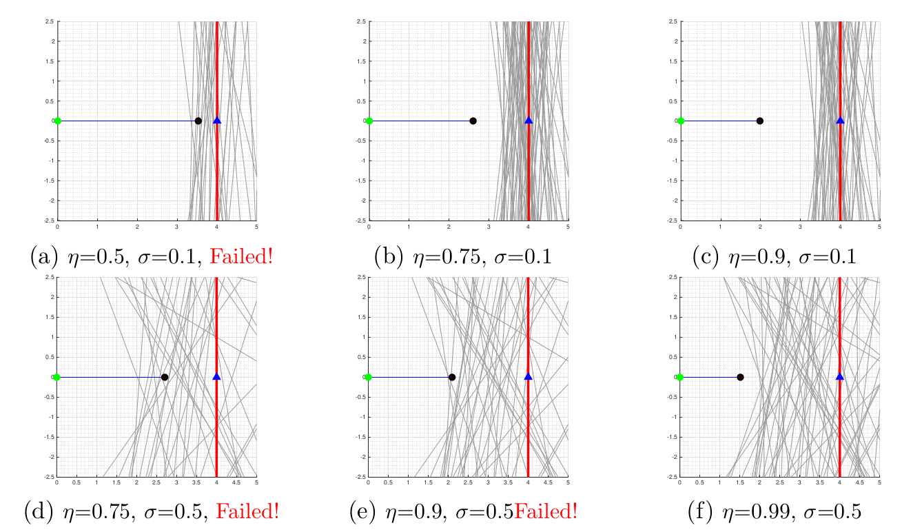
Simulations for various \(\eta\) and \(\Sigma\), the CLF-PrCBF formulation is run for various probabilities \(η \in \{0.5, 0.75, 0.9, 0.99\}\) and different \(\Sigma \in \{0.1, 0.5\}\). As shown in the Figure, the results are expected. Increasing \(\eta\) ensures that the probability for safety is higher and thus the system stabilizes farther from the barrier (more conservative solution). Similarly for higher \(\Sigma\) the system stabilizes farther from the barrier.

References

1. Ames, Aaron D., Samuel Coogan, Magnus Egerstedt, Gennaro Notomista, Koushil Sreenath, and Paulo Tabuada. “Control barrier functions: Theory and applications.” In 2019 18th European control conference (ECC), pp. 3420-3431. IEEE, 2019.