Understanding Differential Flatness for Nonlinear Systems

The words “differential” and “flatness” together might sound a bit bizarre to the ear; however, they form an interesting concept in control theory. It is a property of certain nonlinear systems that makes it easier to work with these systems. In this post, I'll try to present an overview of differential flatness and how it is used for a couple of example systems. 

The earliest references to differential flatness I came across are by Michel Fliess, Jean Lévine, Philippe Martin, Pierre Rouchon.

It says that all the states and the corresponding inputs for a nonlinear system can be computed from a finite set of variables (typically, less than the number of the original states) and their derivatives (up to a finite order) without any integration. These variables are called flat outputs.

Definition[1]: A system

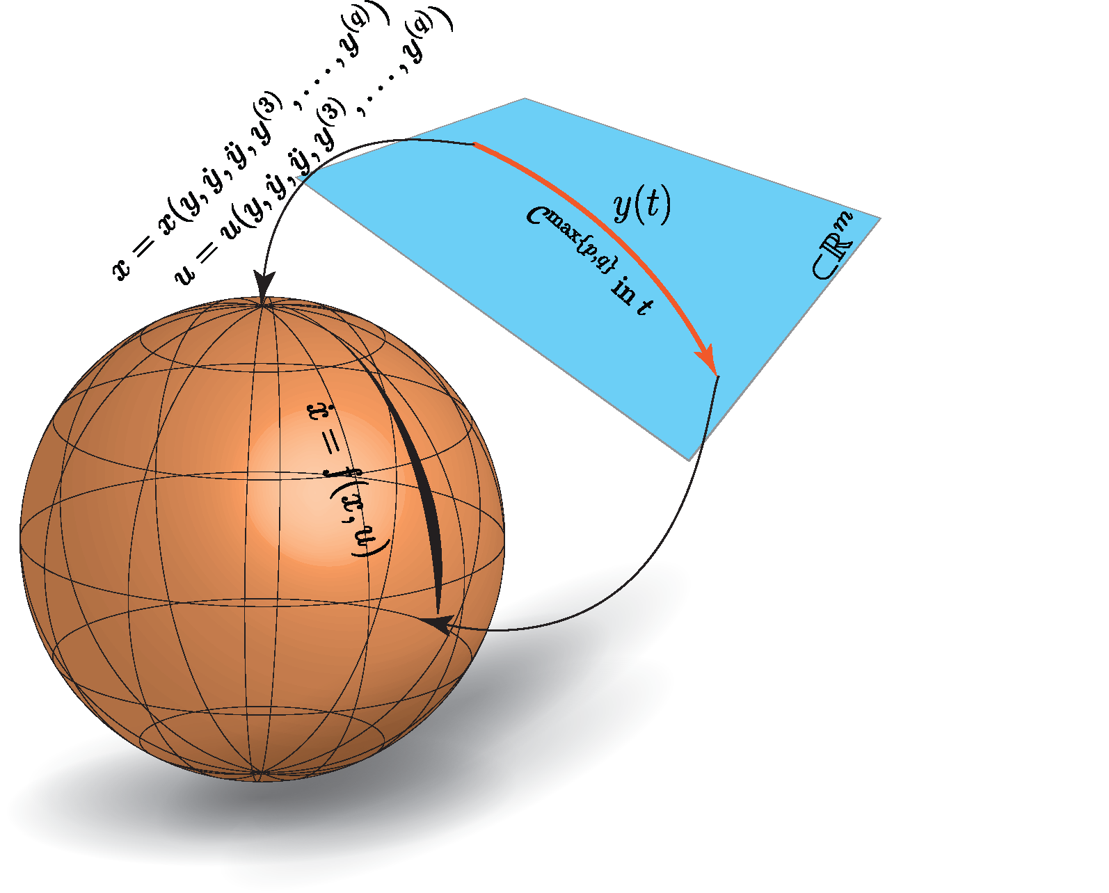
\[ \begin{align} \dot{x}=f(x,u), x\in \mathbb{R}^n, u\in \mathbb{R}^m \end{align} \]

is differentially flat if there exists flat outputs \(y\in \mathbb{R}^m\) of the form \(y=y(x,u,\dot u, \ddot{u}, …, u^{(p)})\) such that the states and the inputs can be expressed as \(x=x(y, \dot{y}, …., y^{(q)})\), \(u = u(y, \dot y, …, y^{(q)})\), where \(p\), \(q\) are positive finite integers.

Note the number of flat outputs is equal to the number of inputs.

Let's look at an obvious example, a double integrator system. The system equations for a double integrator can be written as,

\[ \begin{align} \dot{x} &=v\\ \dot{v} &=u \end{align} \]

For this system, \(x\) is a flat output, i.e., if we know \(x\) as a function of time, then its derivative would give us the \(v\), and the derivative of \(v\) is \(u\). Therefore, knowing \(x\), \(\dot x\), \(\ddot x\), we can have the system states and inputs. Note without any integration from earlier; if we know \(u\) as a function of time, integrating and double integrating would give the states and requires knowing the initial conditions. Keep in mind it is differentially flat and not integrally flat ;). A double integrator system is differentially flat system with \(x\) as the flat output. This example is a bit trivial and might not give more insight into differential flatness.

Now, let's consider an example from [2],

\[ \begin{align} \dot{x}_1 &=x_3-x_2u\\ \dot{x}_2 &=-x_2 + u \\ \dot{x}_3 &=x_2 - x_1 + 2x_2(u-x_2) \end{align} \]

For this system consider a flat output of the form \(y = x_1{ + }\frac{x_2^2}{2}\), taking it derivatives \(\dot y, \ddot y, y^{(3)}\) and solving for \(x_1, x_2, x_3\) gives the system states and inputs (see [2] for details).

\[ \begin{align} x_1 =& -(1+\ddot{y}) + \sqrt{1 + 2 {y} + 2\ddot{y}} \\ x_2 =& \ddot y + x_1 \\ x_3 =& \dot y + {\ddot y }^2 + 2x_1 \ddot y + x_1^2\\ u = & \frac{y^{(3)} + {\ddot y }^2+ \ddot y +\dot y + x_1 + 2x_1\ddot y+ x_1^2 }{1+ \ddot y + x_1} \end{align} \]

These equations seem way more complicated than the original system equations in (4)-(6); why would we want to use them? Well, keep in mind equations (7)-(10) are just expressions for the states and inputs in terms of the flat output \(y\) and its derivatives. i.e., the whole system (4)-(6) behavior can be expressed using a single function \(y(t)\).

How do we make use of this information? We can plan for a desired system behavior by finding a suitable \(y(t)\) with the desired state conditions. For instance, find a \(t\) parameterized curve as,

\[ \begin{align} y = a_0 + a_1 t + a_2 t^ 2 + … + a_p t^p. \end{align} \]

Knowing the desired \(y(t)\), we can find the corresponding system input \(u(t)\). Alternatively, we can use differential flatness as an observer, i.e., by measuring \(y\) we can observe the system states and inputs.

Caveat: Planning in a flat space is not always easy. Sometimes, planning using the full system equations might be easier than planning using the flat outputs. It all depends on how complex and nonlinear the relation between the flat outputs and the system states and inputs is, (7)-(10) for the above example. In the above example, planning in the flat space requires a curve parameterized in \(t\), that's at least three times differentiable, i.e., \(y\in \mathcal{C}^3\). Planning in \(y\) requires at least a \(3^{rd}\) order polynomial or use of periodic function as basis functions. Going more in-depth requires a separate post (see minimum snap/jerk trajectory planning if you are interested). So, for systems that require higher flat-output derivatives (i.e., \(y^{(p)}\)), planning in the flat space might be difficult due to numerical instabilities and/or high computational cost as it requires \(p^{th}\) order polynomial fitting.

Canonical Form

The system in (1) can be expressed in a canonical form using the flat output \(y\) as,

\[ \begin{align} \underbrace{\frac{d}{dt}\begin{bmatrix}y \\ \dot y \\ .\\ . \\ y^{(q-1)} \end{bmatrix}}_{\dot \xi} = \begin{bmatrix} 0 & 1 & 0 & . & 0\\ 0 & 0 & 1 & . & 0\\ . & . & . & . & 0\\ 0 & 0 & 0 & . & 1\\ 0 & 0 & 0 & . & 0 \end{bmatrix} \underbrace{\begin{bmatrix}y \\ \dot y \\ .\\ . \\ y^{(q-1)} \end{bmatrix} }_{\xi} + \begin{bmatrix} 0 \\ 0 \\ .\\ . \\ 1 \end{bmatrix} \underbrace{y^{(q)}}_{\nu} \end{align} \]

the above equation is in the form \(\dot \xi = A \xi + B \nu\) with highest flat output derivative as the virtual input \(\nu\). This is feedback linearization.

For planning using the flat outputs, instead of finding a sufficiently smooth function for \(y(t)\), we can make use of the above canonical form to find \(\nu(t)\) with necessary initial conditions. Trajectory generation techniques like direct collocation, single/multiple shooting methods can be used on the above linear system to find \(y\) and its derivatives.

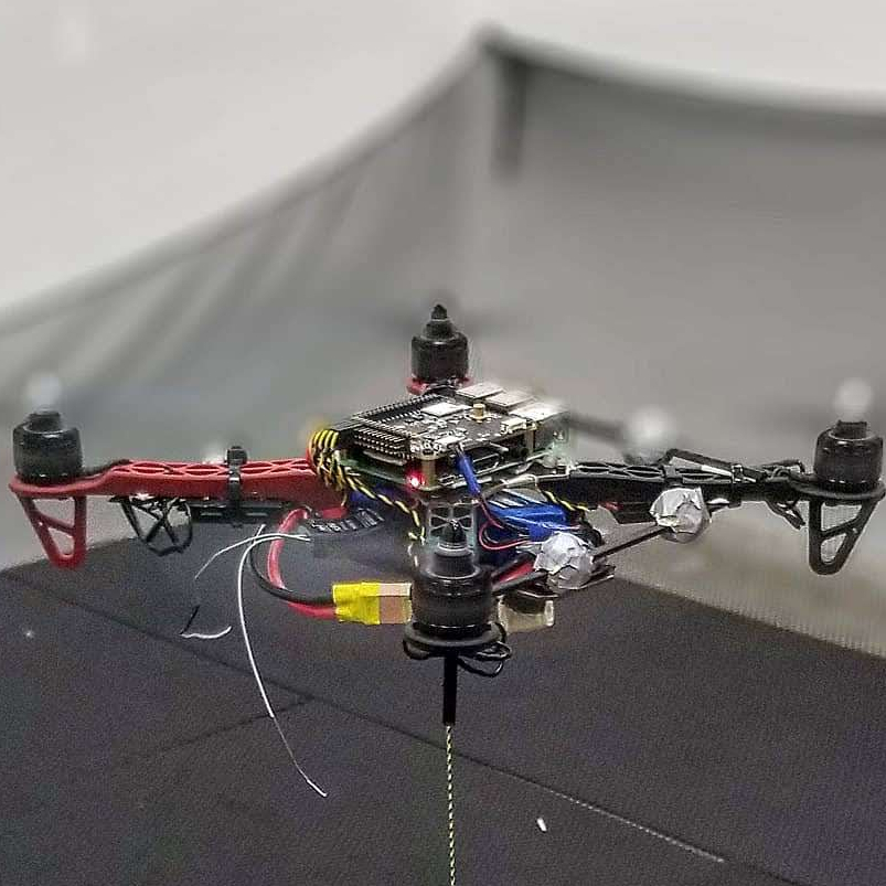
I might have digressed a bit, but I hope you got the idea of using differential flatness for planning. The two earlier examples are a bit abstract; let's look at a more tangible example next, differential flatness in quadrotors and how the states are computed from the flat variables.

References

1. Murray, Richard M., Muruhan Rathinam, and Willem Sluis. “Differential flatness of mechanical control systems: A catalog of prototype systems.” In ASME international mechanical engineering congress and exposition. 1995.

2. Rigatos, Gerasimos G. “Differential flatness theory and flatness-based control.” In Nonlinear Control and Filtering Using Differential Flatness Approaches, pp. 47-101. Springer, Cham, 2015.